Independent Samples t-test with SPSS
Table of Contents
- Example Data, SPSS Data Entry, and Value Labels
- SPSS: Independent Samples t-test Commands
- SPSS: Independent Samples t-test Results
- SPSS: Selecting Two Groups When More than Two Groups Are Present
1. Example Data, SPSS Data Entry, and Value Labels
One may use the independent samples t-test to learn whether two groups have mean scores that differ, statistically, on a quantitative, continuous variable. For example, suppose one is interested in learning whether differences exist between females and males in mathematics scores. Data for such a comparison are presented below in Figure 1.
Figure 1
Mathematics Scores for Females (coded 1 in the Sex column)
and Males (coded 2 in the Sex column)
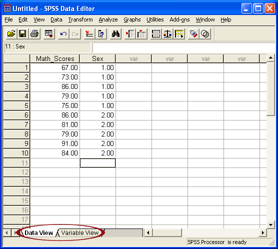
Note the format of data in Figure 1. The first column, labeled Math_Scores contains individual student mathematics scores. The second column, labeled Sex, identifies whether the student is male or female. As noted in Figure 1, females are coded as 1 and males are coded as 2. One may be curious why numbers are used to represent sex when letters such as F and M should suffice. Often statistical programs, such as SPSS, are programmed to work with numbers rather than letters or other symbols. That is the case for the independent samples t-test command in SPSS.
To help users more easily recognize which students are females and males, one may opt to provide Value Labels for the Sex variable. Figure 1 above shows the "Data View" of the SPSS spreadsheet. Note the tab at the bottom of the spreadsheet labeled "Data View." Next to that tab is a second tab labeled "Variable View." Click on "Variable View" to access the variable characteristics section of the spreadsheet.
Figure 2
Variable View Showing Variable Characteristics
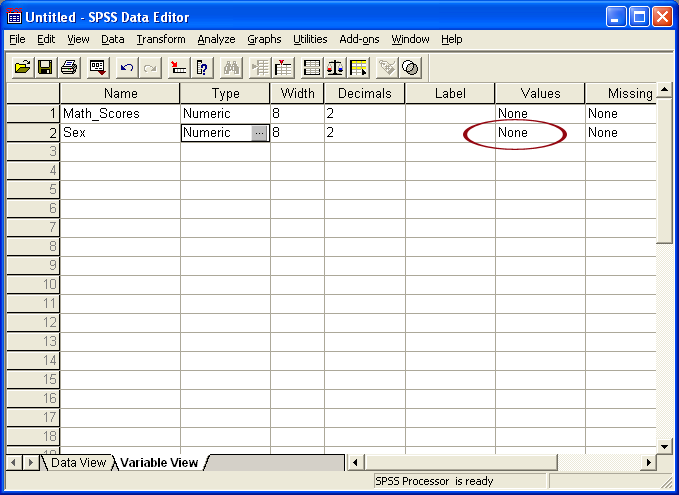
Figure 2 above shows the "Variable View" section of the spreadsheet. Note in Figure 2 the column labeled "Values;" this is the column that allows one to add labels to the values 1 and 2 for Sex. To begin adding labels for the variable Sex, click on the circled cell with "None" entered. The resulting pop-up window is shown in Figure 3 below.
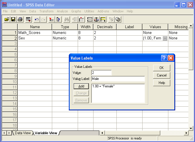
As shown in Figure 3, the label "Female" is added for a Sex value = 1, and the label "Male" will be added for those students with a Sex value = 2. One much click on the "Add" button to complete adding both value labels for sex.
Figure 3
Values Label Pop-up Window
2. SPSS: Independent Samples t-test Commands
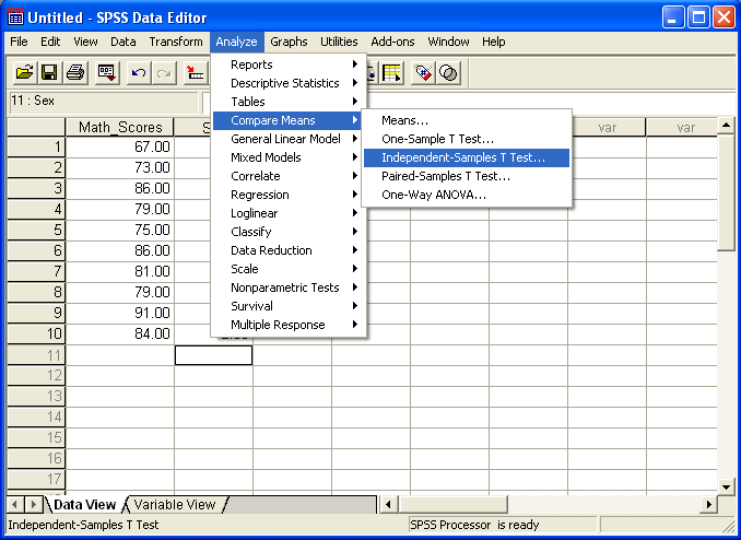
To access the Independent Samples t-test
- select "Analyze"
- select "Compare Means"
- select "Independent Samples t-test"
Figure 4 shows how the current screen should appear.
Figure 4
Accessing Independent Samples t-test Command
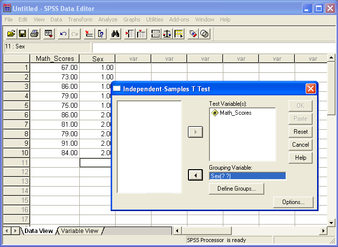
The Independent Samples t-test pop-up window will appear. Select
- the dependent variable (the quantitative variable, mathematics scores in this example) and move it to the "Test Variable(s)" box,
- and move the grouping variable (the categorical independent variable, sex in this example) to the "Grouping Variable" box.
Figure 5 shows the result.
Figure 5
Independent Samples t-test Pop-up Window
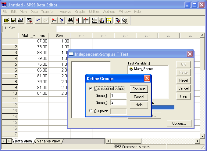
Now the groups must be defined so SPSS correctly compares the two groups of interest (if more than two groups are present in the data). In the current example there are only two groups; to define these
- click on "Define Groups" button,
- identify which group will serve as Group 1 (in this case Females--coded 1-- were selected), then
- identify which group will serve as Group 2 (males coded 2).
- Click "Continue" then click "OK" to run the t-test and obtain results.
The choice of which group will be Group 1 and Group 2 is user defined. If more than two groups are present, the "Define Groups" box enables one to identify which two groups among many will be compared. This option will be illustrated below.
Figure 6
Groups Defined (Identified) for Comparisons
3. SPSS: Independent Samples t-test Results
Presented below are SPSS results for the independent samples t-test.
Figure 7
Results: Descriptive Statistics per Group

Figure 7 presents the two Sex groups, Female and Male. Note the Value Labels added earlier, Female and Male, are displayed in this table under the column labeled Sex rather than the numbers 1 and 2. The table also presents, for both groups, sample sizes (n = 5 each), mean mathematics test scores, standard deviations, and stand errors for the mean.
Figure 8
Results: t-test Results

Figure 8 presents t-test results. To help identify components of this table, each column is numbered in red below the SPSS results in Figure 8. Descriptions of each column are presented below.
Column Descriptions
-
Identifies the dependent variables present. In this example it is "Math_Scores."
-
This column identifies the two rows present, one for "Equal variances assumed" and one for "Equal variances not assumed." More on the equal variances assumption is explained below.
-
One assumption of the t-test is that both groups have equal variances. The t-test is generally robust to this assumption so in most cases t-test results for both rows will lead to the same conclusion. However, occasionally dissimilar variances will be observed which may lead to some differences in t-test results.
-
Levene's Test for Equality of Variances (columns 3 and 4) may be used to test the assumption of equal variances.
-
The value in column 4 is a p-value for Levene's test. This value is labeled "Sig." If this "Sig." value is less that whatever alpha standard one adopts (normally either .10 or .05), then one concludes variances between groups are not equal. If the "Sig." value is larger than the alpha level adopted, then conclude group variances are equal.
-
If group variances are viewed as equal, then use the t-test statistics found on the row entitled "Equal variances are assumed"
-
If group variances are not viewed as equal, then use the t-test statistics found on the row entitled "Equal variances not assumed"
-
-
This column contains the F-ratio for Levene's test of equal variances between groups.
-
Label "Sig.," this column presents the p-value for Levene's test. As noted above, if this value is greater than .10 or .05, then assume groups have equal variances. In this example the groups appear to have similar variances since "Sig." = .437 which is greater than both .10 and .05. Given this result, use "Equal variances assumed" row for t-test results.
-
The t-ratio presented. For the current example, the t-ratio = -2.165.
-
Column contains degrees of freedom (df) for t-test. Current example df = 8
-
The p-value for the t-test is reported as "Sig. (2-tailed)" and is .062 for the current example. If one adopted a Type I error rate (alpha) of .05, then one would fail to reject the null hypothesis of no mean mathematics differences between females and males since .062 > .05.
-
The calculated mean difference between females and males in mathematics scores is -8.20. This value derived from male mean mathematics scores subtracted from females mean mathematics scores: 76.00 - 84.20 = -8.20.
-
Standard error of mean difference. This value, equal to 3.78682 for the current example, is used to calculate confidence interval.
-
The lower limit for the 95% confidence interval.
-
The upper limit for the 95% confidence interval.
4. SPSS: Selecting Two Groups When More than Two Groups Are Present
Suppose one wished to compare two groups, but the data contained more than two groups. Figure 9 shows data for three study groups and mathematics scores.
Figure 9
Three Group Data
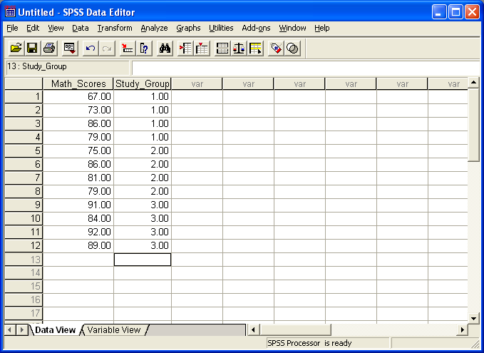
Figure 10 shows the SPSS menu for selecting the t-test command.
Figure 10
Accessing Independent Samples t-test Command
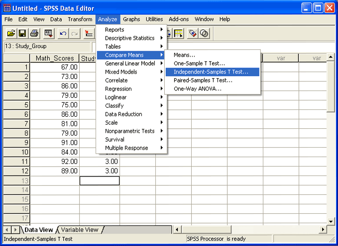
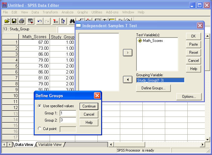
Figure 11 shows how to define which groups will be compared. Select the "Define Groups" button, and enter group numbers for those groups targeted for comparison. Note that groups 1 and 3 were selected for comparison with the example study group data.
Figure 11
Identifying Which Groups to Compare via t-test
Copyright 2010, College of Education, Georgia Southern University
Created by Bryan W. Griffin
Thursday, August 18, 2011
18 August, 2011 11:55 AM