Chi-Square Goodness-of-Fit with SPSS
Table of Contents
A. Purpose of Chi-square Goodness-of-Fit
B. Grouped Data Examples
- Example with Equal Distribution Assumed
- Example with Unequal Distribution Assumed
C. Ungrouped Data Example
A. Purpose of Chi-square Goodness-of-Fit
One may use the chi-square goodness-of-fit test to determine whether a distribution of data or scores for one nominal (categorical)variable matches expectations for that distribution. Consider, for example, the following scenarios:
- In a review admissions policies, administrators at a college wish to know whether male and female students are being admitted with similar frequencies;
- library staff study daily counts of patrons to learn whether number of visitors differ by day of the week, and if some days show heavier counts of patrons than others, then these numbers should be considered when planning staffing needs; and
- if sickness is a random event then one may expect that sick days claimed by employees should be equally distributed among the week (i.e., equal numbers of sick days claimed for Monday, Tuesday, Wednesday, Thursday, and Friday), however, actual counts of sick days may show that some days are claimed more frequently than others (e.g. Friday)--is this discrepancy for high count of sick days on Friday explained by random chance or perhaps by some other factor?
The chi-square goodness-of-fit test can be used to help determine whether distribution of counts in each of the scenarios listed above differ from what one would expect by chance alone.
When performing chi-square goodness-of-fit test one may assume an equal distribution for the counts (i.e., 50% of the students admitted should be female and 50% should be male), or one may assume unequal distributions (i.e., historically 80% of education students are female and 20% male, so recent student admissions should show similar percentages). Finding chi-square goodness-of-fit test results for both equal and unequal distributions are illustrated below.
B. Grouped Data
1. Example with Equal Distribution Assumed
As a simple example for which one would expect equal distributions--equal counts--of results consider 60 rolls of a six-sided die. In theory if a fair die were rolled 60 times, one would expect the following equal frequency distribution displayed in Table 1.
Table 1
Expected Counts for 60 Rolls of a Fair, Six-sided Die
| Die Side | Expected Frequency of Result |
| 1 | 10 |
| 2 | 10 |
| 3 | 10 |
| 4 | 10 |
| 5 | 10 |
| 6 | 10 |
(a) Data Entry in SPSS
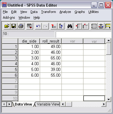
Now suppose this die was rolled 300 times and the results recorded as displayed below in Figure 1. Of interest is whether the results of these 300 die rolls conform with expected results of approximately equal counts for each side of the die. If the observed counts differ from the expected counts of equal distribution for each die side, this may provide evidence that the die is not fair.
In Figure 1 note that the columns labeled "die_side" represents the possible die result and "roll_result" is the count of rolls showing each die side. For example a die roll of 1 occurred 49 times and a die roll of 2 occurred 46 times.
Figure 1
Observed Frequency Results for 300 Rolls of a Six-sided Die
(b) Weight Cases for Grouped Data
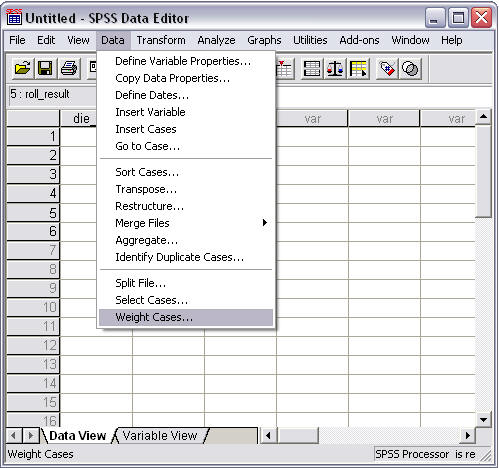
When grouped data are entered in SPSS, that is, when frequencies or counts for each possible category are recorded---die roll numbers from 1 to 6 in this example---one must inform SPSS that counts are used instead of raw, ungroup data. The "Weight Cases" command must be used:
- Select "Data"
- Select "Weight Cases"
Figure 2 shows how the screen should appear upon selecting Data ►Weight Cases.
Figure 2
Weight Cases Command
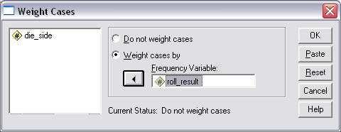
In the pop-up window that appears, select the weighting variable---the frequency of event or count of event variable---and move it to the "Frequency Variable" box as shown below in Figure 3.
Figure 3
Weight Cases Pop-up Window
(c) Chi-square Commands
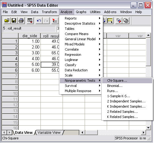
To perform the goodness-of-fit chi-square, run the following commands:
- Select "Analyze"
- Select "Nonparametric Tests"
- Select "Chi-square"
These command selections are illustrated in Figure 4 below.
Figure 4
Chi-square Goodness-of-Fit Selection
With the pop-up window that appears:
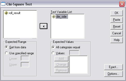
- Move variable to be tested to the "Test Variable List" (which is "die_side" in this example)
- Click "OK" to run the analysis
Note that for "Expected Values" an equal distribution is assumed, i.e., there should be an equal count for each die side because a fair die would produce equal probabilities for each side. In the current example the radio button is marked next to "All categories equal" which informs SPSS that an equal distribution is expected for each side of the die. See Figure 5.
Figure 5
Chi-square Goodness-of-Fit Command
(d) Results
SPSS results for the chi-square goodness-of-fit are provided below in Figure 6.
Figure 6
Chi-square Goodness-of-Fit Results
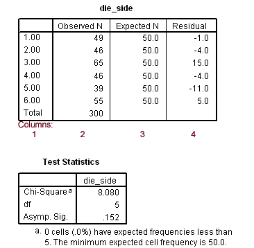
To help identify components of the first table, labeled "die_side" in Figure 6, each column is numbered in red. Descriptions of each column are presented below.
Column Descriptions
-
Identifies the categories of the variable examined (die sides in this example).
-
Observed N: The observed frequencies for the die rolls.
-
Expected N: The expected frequencies of die rolls if all sides are equally likely.
-
Residual: The difference between Observed - Expected. The larger the residual, in absolute value, the greater the discrepancy between observed and expected frequencies. In the current example the roll 3 occurred more often than would be expected by a margin of 15 rolls.
The second table, labeled "Test Statistics" presents three results:
- Chi-square = 8.08: the calculated chi-square value.
- df = 5: the test degrees of freedom.
- Asymp. Sig. = .152: the test p-value.
The p-value for this test is .152; one compares this to alpha which is often set at .05 or .01. If the p-value is less than alpha, reject the null hypothesis that the die produces equal distribution of rolls, and if the p-value is greater than alpha fail to reject the null. In this example the p-value of .152 is larger than .05 so fail to reject the null and conclude that the die appears to produce roll frequencies that are consistent with expectations; the die appears to produce fair rolls.
(e) Remove Weighting
It is important that one removes the weighting effect before proceeding to other analyses otherwise all results calculated will be incorrect. To remove weighting, follow these commands:
- Select "Data"
- Select "Weight Cases"
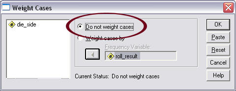
- Place mark next to "Do not weight cases"
See Figure 7 for details.
Figure 7
Removing Weighting
2. Example with Unequal Distribution Assumed
Sometimes one does not expect frequencies, or counts, to be similar for all possible outcomes. Domino's Pizza (Feb. 2011) introduced chicken wings to their menu and asked customers to provide feedback to the following question:
Rate Our Chicken: Did we get it right?
___ Nope
___ Almost
___ Oh Yes We Did
It would be unrealistic to expect 100% of respondents to select the positive "Oh Yes We Did" response. Instead, one may hope that 40% of customers will select the affirmative response, while 35% will select Nope and 25% will select Almost. Thus, the anticipated or targeted proportions of all responses may follow this distribution:
| Nope | = .35 |
| Almost | = .25 |
| Oh Yes We Did | = .40 |
Suppose after testing at one location 211 customers provided feedback with the following counts:
| Nope | = 59 |
| Almost | = 19 |
| Oh Yes We Did | = 133 |
Are these frequencies consistent with expected proportions?
(a) Data Entry in SPSS
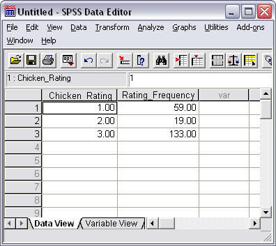
Figure 8 shows how the data may be entered into SPSS. For the "Chicken_Rating" column, the value 1 = Nope, 2 = Almost, and 3 = Oh Yes We Did. The "Rating_Frequency" column indicates customer rating selection counts.
It is very important to recognize and record the numbers assigned to the categories (i.e., 1 = Nope, 2 = Almost, & 3 = Oh Yes We Did) because these numbers will decide how unequal distributional assignments will be determined in SPSS. This is discussed shortly below.
Figure 8
Customer Feedback on Chicken Wing Ratings
(b) Weight Cases for Grouped Data
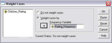
As before, it is necessary to inform SPSS we frequency counts are used for data entry. The "Weight Cases" command must be used:
- Select "Data"
- Select "Weight Cases"
Figure 9 shows how the screen should appear upon selecting "Rating_Frequency" as the weighting variable in the Weight Cases pop-up window.
Figure 9
Weight Cases Command
(c) Chi-square Commands
To perform the goodness-of-fit chi-square, run the following commands:
- Select "Analyze"
- Select "Nonparametric Tests"
- Select "Chi-square"
See Figure 4 above for an illustration.
Once "Chi-square" is selected, a pop-up window will appear. With the pop-up window that appears:
- Move variable to be tested to the "Test Variable List" (which is "Chicken_Rating" in this example)
See Figure 10 below for an illustration.
Figure 10
Chi-square Goodness-of-Fit Selection
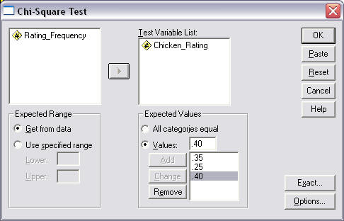
Notice also in Figure 10 the "Expected Values" box. It is with this command area that one sets the expected proportions for the possible outcomes. As previously stated, customer responses are anticipated to following the following proportions of responses:
| Nope | = .35 |
| Almost | = .25 |
| Oh Yes We Did | = .40 |
Two important notes:
- When entering this information into SPSS these proportions must sum to 1.00 to account for 100% of responses otherwise an incorrect chi-square value will be calculated.
- It is critical that the proportions entered match the category numbers assigned; category 1 = "Nope" is .35, category 2 = "Almost" is .25, and category 3 = "Oh Yes We Did" is .40, so proportions must be entered in this order: .35, .25, then .40.
As a second example of the proportion order, suppose the category numbers were changed as follows: category 3 = "Nope" with proportion of .35, category 2 = "Almost" with proportion of .25, and category 1 = "Oh Yes We Did" with proportion of .40. The order of entry in SPSS of the proportions now must be .40 (for category 1), .25 (for category 2), and .35 (for category 3).
To run the analysis, click "OK."
(d) Results
SPSS results for the chi-square goodness-of-fit are provided below in Figure 11.
Figure 11
Chi-square Goodness-of-Fit Results for the Chicken Ratings
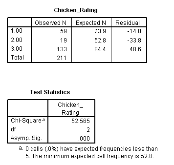
The figure above shows two tables. The first provides the three chicken rating outcomes (1, 2, and 3), the observed frequencies for each (59, 19, and 133), the expected frequencies of each, and the residuals (difference between observed - expected frequencies).
The chi-square value is provided in the second table (chi-square = 52.565), degrees of freedom (df = 2), and p-value for the test result (Asymp. Sig. = p-value = .000).
These results suggest that the observed frequencies do not match well the expected proportions (p < .01), and it seems many more respondents provided a rating of 3 ("Oh Yes We Did") that was anticipated.
(e) Remove Weighting
As previously noted, it is important that one remove the weighting effect before proceeding to other analyses:
- Select "Data"
- Select "Weight Cases"
- Place mark next to "Do not weight cases"
See Figure 7, above, for and example.
C. Ungrouped Data Example
Often one may have raw, ungrouped data for analysis. For example, suppose one wishes to know whether class enrollment by sex (female vs. male) differs from a 50:50 ratio.
(a) Data Entry in SPSS
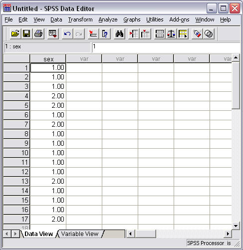
Below are class observations per pupil with a total class size of n = 17 where the recorded categories are 1 = "female" and 2 = "male" (see Figure 12). These data could be tallied to form grouped data for chi-square analysis like illustrated above (in this case there are 12 females and 5 males), or these raw, ungrouped data could be analyzed using chi-square goodness-of-fit.
Figure 12
Student Sex (1 = Female, 2 = Male)
(b) Chi-square Commands
Since raw data will be used, SPSS automatically determines frequencies so there is no need to use the "Weight Cases" command. Instead, one may move directly to the chi-square command:
- Select "Analyze"
- Select "Nonparametric Tests"
- Select "Chi-square"
See Figure 4 above for an illustration.
Once "Chi-square" is selected, a pop-up window will appear. With the pop-up window that appears:
- Move variable to be tested to the "Test Variable List" (which is "Sex" in this example)
See Figure 13 below for an illustration.
Figure 13
Chi-square Goodness-of-Fit for Sex Variable
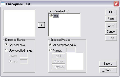
In the above example one may leave the "All categories equal" option marked if one believes the two sexes should be equally distributed within the class (1-to-1 ratio; 50% each), or select appropriate weighting if one thinks one sex would be more likely (e.g., 80% female and 20% male if a College of Education class; since 1 = "female" and 2 = "male", the proportions entered would be .80 then .20).
To run the analysis, click "OK."
(d) Results
SPSS results for the chi-square goodness-of-fit test for student sex are provided below in Figure 14.
Figure 14
Chi-square Goodness-of-Fit Results for Student Sex
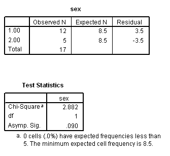
The figure above shows two tables. The first provides the two sex categories (1 = "female", 2 = "male") with 12 females and 5 males reported, and expected frequencies of 8.5 students each (since equal distribution was assumed).
The second table shows the chi-square value 2.882 with df = 1 and p = 0.090. With this example one would conclude the observed student sex distribution could be the result chance variation, i.e., the departure from 50% female and 50% male may be due to random chance.
Copyright 2010, College of Education, Georgia Southern University
Created by Bryan W. Griffin
Thursday, August 18, 2011
18 August, 2011 11:54 AM