Logic of Hypothesis Testing

“Could the results of this study be due to random differences caused by sampling error or by a real effect?”

This is the question addressed in statistical hypothesis testing. To understand the logic used in hypothesis testing that allows one to address this question, the following information is provided.

1. Hypothesis testing is designed around random sampling.

Statistical hypotheses require the assumption that any difference between sample statistics and the population parameters the statistics estimate is due to sampling error and not to bias in the sample. Random difference means that the sample statistic will either randomly over-estimate the parameter (it will be larger than the parameter) or it will randomly under-estimate the parameter (it will be smaller than the parameter). Sampling error represents any random difference between a statistic and its corresponding parameter. If there is a systematic difference that is not due to random fluctuations, then hypothesis testing will be incorrect because the probabilities used in hypothesis testing (discussed below) will be inaccurate.

2. If a distribution of scores is known, then one can calculate the probability of a given score occurring. 

For example, if one knows that the distribution of SAT verbal scores is normally distributed with a mean of 500 and standard deviation of 100, then SAT scores can be converted to Z scores and one can use a Z table to find probabilities. Thus, what is the probability of obtaining an SAT score of 600 or better? Z = [(600-500)/100] = 1, so the probability of getting a Z score of 1 or greater is .1587, or 15.87%.

3. All statistics have a theoretically known distribution and this distribution is called a sampling distribution.

If one collects lots of scores, such as 1000 scores on the verbal SAT, one could plot this distribution of scores with a histogram to determine the shape of the distribution (it would probably be close to normal in shape). A distribution of raw scores like the one described with SAT scores is called a raw score distribution, a distribution of scores, or a sample distribution. Suppose instead that one took 1000 samples of size 30 (that is, one took a sample of 30 SAT scores, and did this 1000 times), calculated the mean for each sample, then plotted the sample means with a histogram. The resulting distribution would be called a sampling distribution (of means). If one viewed this histogram of the sampling distribution, the histogram would show a distribution that is very close to normal in shape. Other statistics have sampling distributions with shapes other than normal, such as the t, F, and chi-square distributions, which are positively skewed distributions.

4. Sampling distributions have means and standard deviations (which are called standard errors).

Since the sampling distribution for a given statistic (such as the mean) is known, one can calculate the probability of getting a statistic of a given size. For example, suppose we have 1000 samples taken from SAT verbal scores. Each sample was of size 30. For each sample the mean is calculated and then these means are used to form the sampling distribution. One could also calculate the standard deviation for these means, since there will be variability in the means (i.e., the means will not all be the same). This standard deviation of the means is given a special name, the standard error of the mean. In addition to the standard error of the mean, one could also calculate the mean of the sampling distribution. This mean will be a mean of means—that is, since the sampling distribution in this example is of sample means, one could calculate the mean of the means. This mean of the means will be equal to the population mean, the parameter. So two things: (a) the sampling distribution has a standard deviation and it is called the standard error; (b) the sampling distribution of sample means also has a mean and this mean is equal to the population mean (the parameter).

5. Hypothesis testing assumes the null hypothesis (Ho) is true.

Null hypotheses vary by the type of data and statistical test used, but in all cases the null hypothesis is assumed to be true when calculating information to perform a statistical test of the null. Consider one of the more simplistic statistical tests, the one-group t-test. In this test, one compares a sample mean to a set value. For example, one may wish to know if a sample of students applying for admission to a given college is different from the national average. For SAT verbal scores, the national average mean is 500. Suppose a sample of 30 students who applied for admission to this college had an average SAT verbal score of 488, thus a 12 point difference from the national average, 488-500 = -12. The null hypothesis is symbolized as follows:

Ho: m = 500

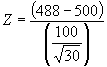
Thus, the null states that there is no difference between the population represented by the college’s sample (the population here is defined as all students who apply for admission to this college) and the national average score for all students who took the SAT verbal section. If the assumption of the null is correct, then one is able to calculate the probability of obtaining a sample mean that is as discrepant as the one obtained in the sample. In other words, one can calculate the probability of getting a sample average score that is 488 or lower for a population in which the true mean is 500. How is this calculated? Since (a) the distribution of means is known to approximate a normal distribution, (b) the population mean (500 in this case) is known, and (c) the standard error is known, one could convert the mean score of 488 into a Z score and reference the Z table to find associated probabilities. The Z score for 488 could be:

= -12/18.25 = -.66. The probability of obtaining a Z score this small or smaller is .2546 or 25.46% of the time. So one could expect to obtain a sample mean score of 488 or smaller about 25% of the time if random samples were repeated infinitely.

6. Hypotheses are judged by p-values.

The probability value calculated above based upon the sampling distribution is referred to as a p-value. As noted above, the p-value for the mean score of 488 is .2546 and this indicates that one could expect to find a mean score of 488, or lower, from a sample of size 30 about 25% of the time with random samples if the null hypothesis is true (i.e., that our sample does not come from a population that differs from the population with a mean score of 500).

In hypothesis testing convention holds that if the calculated p-value is small enough, one has evidence to conclude that the sample differs from the population specified in the null. For example, the null in the SAT example used here is that there is no difference between the mean SAT score for the sample of 30 students selected and the national average SAT score of 500. With a score of 488 and a p-value of .25, it seems likely that –12 point difference is the result of random sampling difference, or sampling error, and not due to real differences between the sample selected and the national population SAT average. However, suppose that the sample selected demonstrated a mean difference of 50 points, i.e., mean score of 450. The probability of obtaining a sample mean this small or smaller at random is much lower. First, the Z score is:

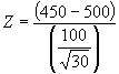
= -50/18.25 = -2.74, and the corresponding p-value (obtained from the Z table) is .003. This p-value indicates that if the null hypothesis is true and the sample of students applying to this college is the same as students nationwide, then would one could expect to get a sample mean of 450, or lower, about 3 times out of 1,000 random samples.

When the p-value is small, one has a decision to make. Either the sample has much sampling error thus distorting the true image of the population (a 450 mean vs. a 500 mean), OR the sample actually represents a different population that is not consistent with the hypothesized population. In other words, either this sample data comes from outliers and is a fluke, or this sample represents a group of people who are different from the typical population. In hypothesis testing, usually the null hypothesis is rejected if the p-value is less than .05 or .01. If the hypothesis about the SAT scores is rejected, then one is concludes that this particular sample of students represents students who are different from the population on the whole and appears to represent a population of student for which lower SAT scores are the norm.

7. p-value reflect either directional or non-directional tests.

To be covered in class.

8. Errors in Hypothesis Testing

In hypothesis testing, two decisions can be made, either reject H0 or fail to reject H0. Two errors can also be made in deciding whether to reject or fail to reject H0. The table below specifies each of these errors.

Note that the probabilities of each outcome are given in parentheses.

Case 1: Reject H0 when H0 is true.

This is an error because the null was rejected and it should not have been rejected. This is a Type I error (rejecting H0 when H0 is true). The probability of making this type of error is equal to , the alpha level that the researcher sets, which is traditionally set at .05 or .01 (and sometimes .10).

Case 2: Fail to reject H0 when H0 is false (H1 is true).

This is also an error, and is known as a Type II error (failing to reject H0 when H0 is false). This error occurs when one does not reject the null hypothesis when it should have been rejected because there really are differences (thus the alternative hypothesis is actually true). The probability of making this type of error is equal to ; unlike , the researcher cannot directly set the level of , but must manipulate other factors which influence  like sample size and/or the alpha level.

Case 3: Reject H0 when H0 is false (H1 is true).

This is a correct decision because H0 is not true so we adopt the alternative hypothesis, H1. The probability of this occurring is 1 - , and this probability is called power.

Case 4: Fail to reject H0 when H0 is true.

This is also a correct decision because H0 was not rejected, and no differences actually exist. The probability of this occurring is 1 - .

The researcher only has direct control of the  error level. The researcher cannot directly manipulate the  error level; however, several factors can increase or decrease . These factors include sample size, the alpha level, type of hypothesis, and the amount of variability in the study. These factors are discussed in more detail below.

9. Power (and Factors that Impact Upon It)

(a) Power Described

Errors in hypothesis testing include the Type I error (rejecting H0 when H0 is true) and the Type II error (failing to reject H0 when H0 is false). The probability of a Type I error is  and is set directly by the researcher. The probability of a Type II error is  and is controlled indirectly by factors that influence the power to the test.

The power of a test is the probability of rejecting a false H0, p(rejecting false H0); the probability of detecting differences if they actually exist. Power is influenced by (a) effect size, (b) n, (c) control of the variability in studies, (d) choice of hypotheses, and (e) -level.

(b) Factors Affecting Power

Effect Size

For a Z test (or one sample t test, discussed later) the size of the difference between the true value of m and that value tested in H0 (M) is referred to as the effect size (ES). For example, suppose one wanted to test the difference in IQ of this statistics class vs. the national average. The average IQ in the statistics class is 130. One simple measure of effect size is 130 - 100 = 30. If, however, the average IQ in the statistics class was 105, then the effect size would be 105 - 100 = 5.

In general, the larger the effect size the more power the test has for detecting differences. If there are large differences, it will be easier to find them (i.e., easier to reject H0). But if there are small differences, it will be more difficult to find them (i.e., more difficult to reject H0).

(Explain why larger ESs provide more power.)

Sample Size

In general, the larger the sample size (n), the more powerful the test. Why does increasing n increase power? Recall that the formula for the standard error of the mean is , so it is easy to see that as n increases, the standard error decreases. Since the standard error is the denominator in the z-score formula for the sample mean, , as the sample size increases, so will  for given sample mean. So how does a change in  affect power? Recall the decision rule:

If      or     , then reject H0; otherwise, fail to reject H0

So as the sample size increases,  will become larger (in absolute value), and this increases the probability of rejecting H0, therefore power is increased.

(Explain why increases in n increases power.)

Variability in Studies

Smaller variability yields larger power. As the population variance, , decreases, power increases. Using the same logic as above, note the formula for the standard error for the sample mean is , so it is easy to see that as   decreases, the standard error will decrease. Since the standard error is the denominator in the z-score formula for the sample mean, , as  decreases, the z-score for sample means will increase in absolute value. So how does this affect power? Recall the decision rule:

If      or     , then reject H0; otherwise, fail to reject H0

So as the  decreases, the absolute value of  becomes larger, and this increases the probability of rejecting H0, so power is increased.

(Explain why decreases in variability increases power.)

Choice of Hypotheses

Directional hypotheses give more power than non-directional hypotheses if the prediction of direction is correct, but directional hypotheses provide zero power if the prediction of direction is incorrect. 

This relationship can be shown as follows. If the researcher sets  = .05, then for a two-tailed (non-directional) test the critical values are 1.96 and -1.96. For a one-tailed (upper-tailed) test, however, the critical value is 1.64 for  = .05. 

So, if one calculates a z-score for a sample mean and it equals, say, 1.78 (i.e.,  = 1.78), then which test is more powerful, the two-tail or one-tailed test? 

With the two-tailed test, H0 would not be rejected since 1.78 does not fall within the rejection region (i.e, 1.78 is not greater than 1.96 or less than -1.96). However, with the one-tailed test H0 is rejected because the obtained z score, 1.78, lies within the rejection region (i.e, 1.78 > 1.64). So directional hypotheses are more powerful because their critical values are smaller than the corresponding critical values of non-directional tests.

(Explain why directional tests are more powerful than non-directional tests. Are directional tests always more powerful; if not, under what circumstances are they less powerful?)

Alpha ( )

The larger the a, the greater the power. That is, the greater the probability of rejecting a false H0, the greater the chance of finding a difference (accepting H1). 

As  becomes larger, say from .01 to .05, one should easily see that it will be easier to reject H0, and since it is easier to reject H0, power is increased. For example, the critical value for a one-tailed test with a = .01 is 2.32, but increasing  to .05 results in a critical value of 1.64. Since the critical z’s, , are smaller with larger ’s, smaller calculated ’s are needed to reject H0. In short, larger ’s result in more power.

(Why does increasing alpha provide increased power?)

Which Factors to Alter?

To increase power, the easiest factors for the researcher to manipulate are n and , but  is usually set at .10, .05, and .01 by tradition. In some circumstances one may also be able to choose directional tests.

Copyright © 2003, Bryan W. Griffin

Last revised on 16 January, 2003 05:57 PM